Stockwell

Python package for time-frequency analysis through Stockwell transform.

Based on original code from NIMH MEG Core Facility.

Installation

Using Anaconda

If you use Anaconda, the latest release of Stockwell is available via
conda-forge.

To install, simply run:

conda install -c conda-forge stockwell

Using pip and PyPI

The latest release of Stockwell is available on the
Python Package Index.

You can install it easily through pip:

pip install stockwell

Installation from source

If no precompiled package is available for you architecture on PyPI, or if you
want to work on the source code, you will need to compile this package from
source.

To obtain the source code, download the latest release from the
releases page, or clone the GitHub project.

C compiler

Part of Stockwell is written in C, so you will need a C compiler.

On Linux (Debian or Ubuntu), install the build-essential package:

sudo apt install build-essential

On macOS, install the XCode Command Line Tools:

xcode-select --install

On Windows, install the Microsoft C++ Build Tools.

FFTW

To compile Stockwell, you will need to have FFTW
installed.

On Linux and macOS, you can download and compile FFTW from source using
the script get_fftw3.sh provided in the scripts directory:

./scripts/get_fftw3.sh

Alternatively, you can install FFTW using your package manager:

• If you use Anaconda (Linux, macOS, Windows):

  conda install fftw
  

• If you use Homebrew (macOS)

  brew install fftw
  

• If you use apt (Debian or Ubuntu)

  sudo apt install libfftw3-dev
  

Install the Python package from source

Finally, install this Python package using pip:

pip install .

Or, alternatively, in "editable" mode:

pip install -e .

Usage

Example usage:

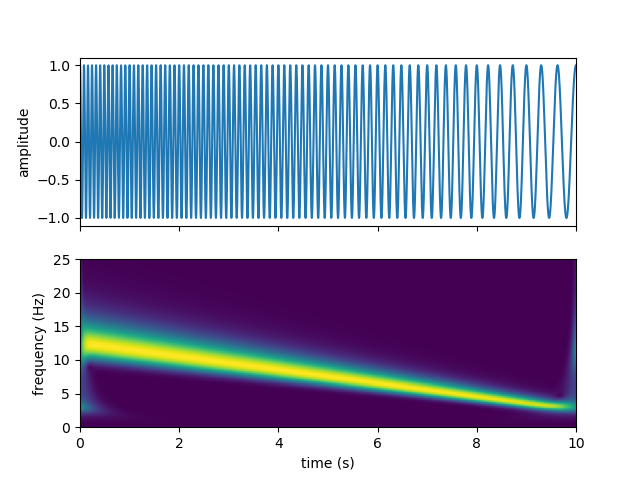
pythonCopy
import numpy as np
from scipy.signal import chirp
import matplotlib.pyplot as plt
from stockwell import st

t = np.linspace(0, 10, 5001)
w = chirp(t, f0=12.5, f1=2.5, t1=10, method='linear')

fmin = 0  # Hz
fmax = 25  # Hz
df = 1./(t[-1]-t[0])  # sampling step in frequency domain (Hz)
fmin_samples = int(fmin/df)
fmax_samples = int(fmax/df)
stock = st.st(w, fmin_samples, fmax_samples)
extent = (t[0], t[-1], fmin, fmax)

fig, ax = plt.subplots(2, 1, sharex=True)
ax[0].plot(t, w)
ax[0].set(ylabel='amplitude')
ax[1].imshow(np.abs(stock), origin='lower', extent=extent)
ax[1].axis('tight')
ax[1].set(xlabel='time (s)', ylabel='frequency (Hz)')
plt.show()

You should get the following output:

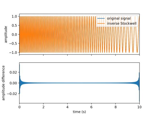
You can also compute the inverse Stockwell transform, ex:

pythonCopy
inv_stock = st.ist(stock, fmin_samples, fmax_samples)
fig, ax = plt.subplots(2, 1, sharex=True)
ax[0].plot(t, w, label='original signal')
ax[0].plot(t, inv_stock, label='inverse Stockwell')
ax[0].set(ylabel='amplitude')
ax[0].legend(loc='upper right')
ax[1].plot(t, w - inv_stock)
ax[1].set_xlim(0, 10)
ax[1].set(xlabel='time (s)', ylabel='amplitude difference')
plt.show()

References

Stockwell, R.G., Mansinha, L. & Lowe, R.P., 1996. Localization of the complex
spectrum: the S transform, IEEE Trans. Signal Process., 44(4), 998–1001,
doi:10.1109/78.492555

S transform on Wikipedia.