correlation <img src='man/figures/logo.png' align="right" height="139" />

correlation is an
easystats package focused
on correlation analysis. It’s lightweight, easy to use, and allows for
the computation of many different kinds of correlations, such as
partial correlations, Bayesian correlations, multilevel
correlations, polychoric correlations, biweight, percentage
bend or Sheperd’s Pi correlations (types of robust correlation),
distance correlation (a type of non-linear correlation) and more,
also allowing for combinations between them (for instance, Bayesian
partial multilevel correlation).

Citation

You can cite the package as follows:

Makowski, D., Ben-Shachar, M. S., Patil, I., & Lüdecke, D. (2020).
Methods and algorithms for correlation analysis in R. Journal of Open
Source Software, 5(51), 2306. https://doi.org/10.21105/joss.02306

Makowski, D., Wiernik, B. M., Patil, I., Lüdecke, D., & Ben-Shachar, M.
S. (2022). correlation: Methods for correlation analysis [R
package]. https://CRAN.R-project.org/package=correlation (Original
work published 2020)

Installation

The correlation package is available on CRAN, while its latest
development version is available on R-universe (from rOpenSci).

Type	Source	Command
Release	CRAN	install.packages("correlation")
Development	R-universe	install.packages("correlation", repos = "https://easystats.r-universe.dev")

Once you have downloaded the package, you can then load it using:

rCopy
library("correlation")

Tip

Instead of library(bayestestR), use library(easystats). This will
make all features of the easystats-ecosystem available.

To stay updated, use easystats::install_latest().

Documentation

Check out package website
for documentation.

Features

The correlation package can compute many different types of
correlation, including:

✅ Pearson’s correlation<br> ✅ Spearman’s rank correlation<br>
✅ Kendall’s rank correlation<br> ✅ Biweight midcorrelation<br>
✅ Distance correlation<br> ✅ Percentage bend correlation<br>
✅ Shepherd’s Pi correlation<br> ✅ Blomqvist’s coefficient<br>
✅ Hoeffding’s D<br> ✅ Gamma correlation<br> ✅ Gaussian rank
correlation<br> ✅ Point-Biserial and biserial correlation<br> ✅
Winsorized correlation<br> ✅ Polychoric correlation<br> ✅
Tetrachoric correlation<br> ✅ Multilevel correlation<br>

An overview and description of these correlations types is available
here.
Moreover, many of these correlation types are available as partial
or within a Bayesian framework.

Examples

The main function is
correlation(),
which builds on top of
cor_test()
and comes with a number of possible options.

Correlation details and matrix

rCopy
results <- correlation(iris)
results
## # Correlation Matrix (pearson-method)
## 
## Parameter1   |   Parameter2 |     r |         95% CI | t(148) |         p
## -------------------------------------------------------------------------
## Sepal.Length |  Sepal.Width | -0.12 | [-0.27,  0.04] |  -1.44 | 0.152    
## Sepal.Length | Petal.Length |  0.87 | [ 0.83,  0.91] |  21.65 | < .001***
## Sepal.Length |  Petal.Width |  0.82 | [ 0.76,  0.86] |  17.30 | < .001***
## Sepal.Width  | Petal.Length | -0.43 | [-0.55, -0.29] |  -5.77 | < .001***
## Sepal.Width  |  Petal.Width | -0.37 | [-0.50, -0.22] |  -4.79 | < .001***
## Petal.Length |  Petal.Width |  0.96 | [ 0.95,  0.97] |  43.39 | < .001***
## 
## p-value adjustment method: Holm (1979)
## Observations: 150

The output is not a square matrix, but a (tidy) dataframe with all
correlations tests per row. One can also obtain a matrix using:

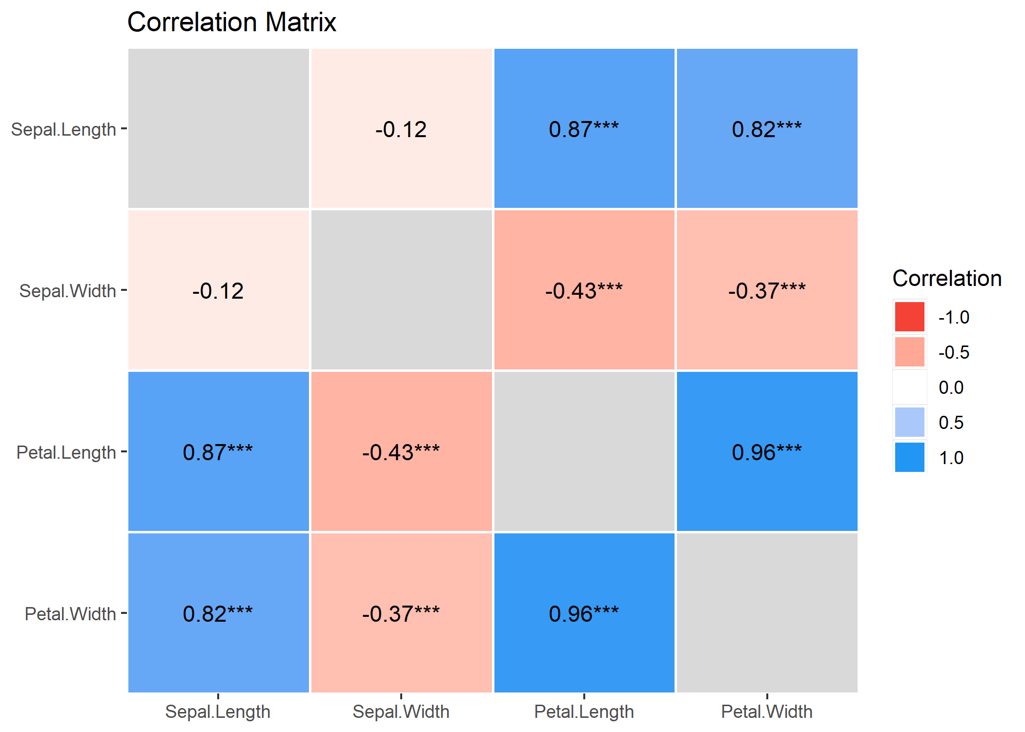
rCopy
summary(results)
## # Correlation Matrix (pearson-method)
## 
## Parameter    | Petal.Width | Petal.Length | Sepal.Width
## -------------------------------------------------------
## Sepal.Length |     0.82*** |      0.87*** |       -0.12
## Sepal.Width  |    -0.37*** |     -0.43*** |            
## Petal.Length |     0.96*** |              |            
## 
## p-value adjustment method: Holm (1979)

Note that one can also obtain the full, square and redundant matrix
using:

rCopy
summary(results, redundant = TRUE)
## # Correlation Matrix (pearson-method)
## 
## Parameter    | Sepal.Length | Sepal.Width | Petal.Length | Petal.Width
## ----------------------------------------------------------------------
## Sepal.Length |              |       -0.12 |      0.87*** |     0.82***
## Sepal.Width  |        -0.12 |             |     -0.43*** |    -0.37***
## Petal.Length |      0.87*** |    -0.43*** |              |     0.96***
## Petal.Width  |      0.82*** |    -0.37*** |      0.96*** |            
## 
## p-value adjustment method: Holm (1979)

rCopy
library(see)

results %>%
  summary(redundant = TRUE) %>%
  plot()

<!-- -->

Correlation tests

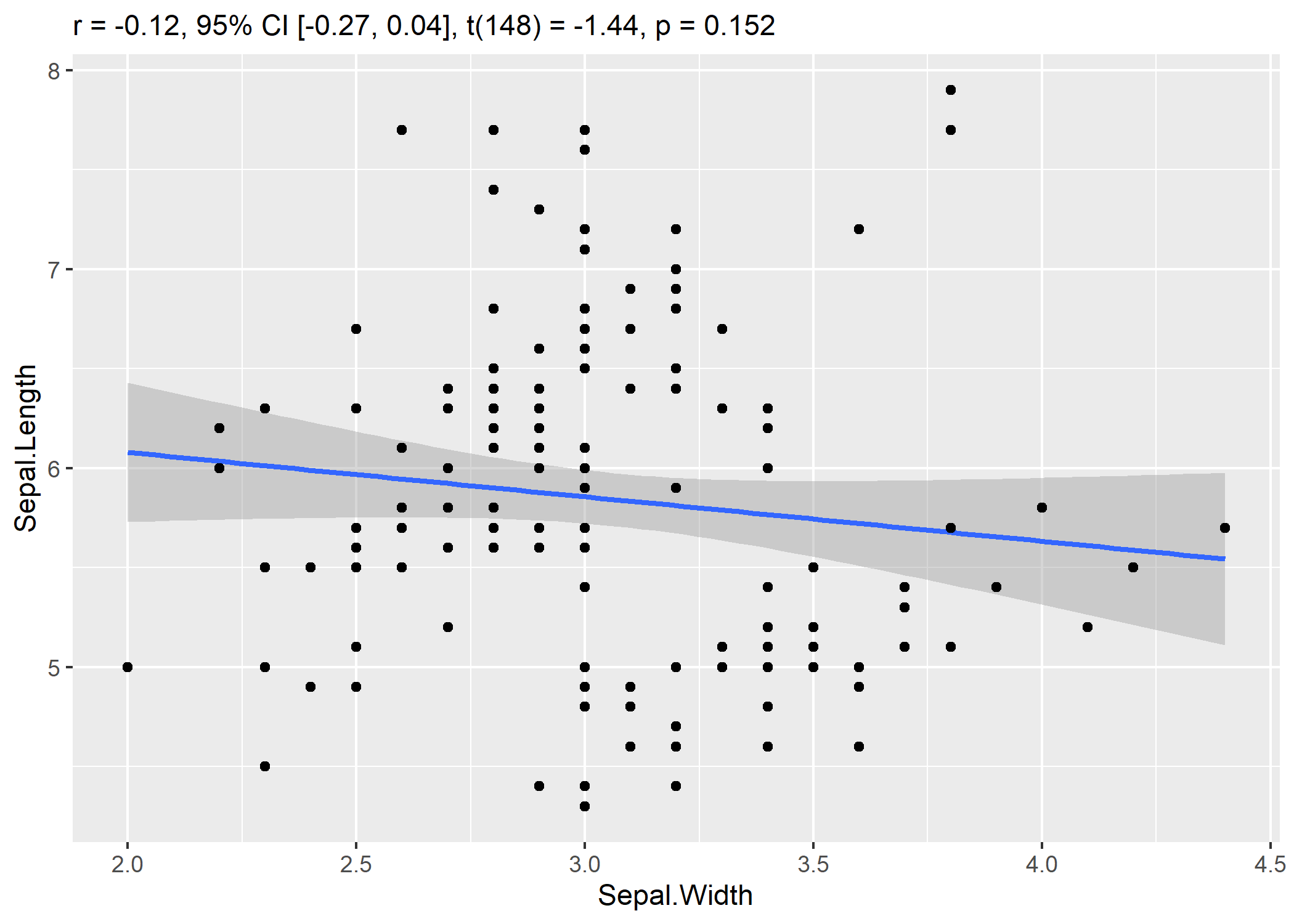
The cor_test() function, for pairwise correlations, is also very
convenient for making quick scatter plots.

rCopy
plot(cor_test(iris, "Sepal.Width", "Sepal.Length"))

<!-- -->

Grouped dataframes

The correlation() function also supports stratified correlations,
all within the tidyverse workflow!

rCopy
iris %>%
  select(Species, Sepal.Length, Sepal.Width, Petal.Width) %>%
  group_by(Species) %>%
  correlation()
## # Correlation Matrix (pearson-method)
## 
## Group      |   Parameter1 |  Parameter2 |    r |        95% CI | t(48) |         p
## ----------------------------------------------------------------------------------
## setosa     | Sepal.Length | Sepal.Width | 0.74 | [ 0.59, 0.85] |  7.68 | < .001***
## setosa     | Sepal.Length | Petal.Width | 0.28 | [ 0.00, 0.52] |  2.01 | 0.101    
## setosa     |  Sepal.Width | Petal.Width | 0.23 | [-0.05, 0.48] |  1.66 | 0.104    
## versicolor | Sepal.Length | Sepal.Width | 0.53 | [ 0.29, 0.70] |  4.28 | < .001***
## versicolor | Sepal.Length | Petal.Width | 0.55 | [ 0.32, 0.72] |  4.52 | < .001***
## versicolor |  Sepal.Width | Petal.Width | 0.66 | [ 0.47, 0.80] |  6.15 | < .001***
## virginica  | Sepal.Length | Sepal.Width | 0.46 | [ 0.20, 0.65] |  3.56 | 0.002**  
## virginica  | Sepal.Length | Petal.Width | 0.28 | [ 0.00, 0.52] |  2.03 | 0.048*   
## virginica  |  Sepal.Width | Petal.Width | 0.54 | [ 0.31, 0.71] |  4.42 | < .001***
## 
## p-value adjustment method: Holm (1979)
## Observations: 50

Bayesian Correlations

It is very easy to switch to a Bayesian framework.

rCopy
correlation(iris, bayesian = TRUE)
## # Correlation Matrix (pearson-method)
## 
## Parameter1   |   Parameter2 |   rho |         95% CI |      pd | % in ROPE
## --------------------------------------------------------------------------
## Sepal.Length |  Sepal.Width | -0.11 | [-0.27,  0.04] |  92.70% |    42.83%
## Sepal.Length | Petal.Length |  0.86 | [ 0.82,  0.90] | 100%*** |        0%
## Sepal.Length |  Petal.Width |  0.81 | [ 0.75,  0.86] | 100%*** |        0%
## Sepal.Width  | Petal.Length | -0.41 | [-0.55, -0.28] | 100%*** |        0%
## Sepal.Width  |  Petal.Width | -0.35 | [-0.49, -0.22] | 100%*** |        0%
## Petal.Length |  Petal.Width |  0.96 | [ 0.95,  0.97] | 100%*** |        0%
## 
## Parameter1   |         Prior |          BF
## ------------------------------------------
## Sepal.Length | Beta (3 +- 3) |       0.509
## Sepal.Length | Beta (3 +- 3) | 2.14e+43***
## Sepal.Length | Beta (3 +- 3) | 2.62e+33***
## Sepal.Width  | Beta (3 +- 3) | 3.49e+05***
## Sepal.Width  | Beta (3 +- 3) | 5.29e+03***
## Petal.Length | Beta (3 +- 3) | 1.24e+80***
## 
## Observations: 150

Tetrachoric, Polychoric, Biserial, Biweight…

The correlation package also supports different types of methods,
which can deal with correlations between factors!

rCopy
correlation(iris, include_factors = TRUE, method = "auto")
## # Correlation Matrix (auto-method)
## 
## Parameter1         |         Parameter2 |     r |         95% CI | t(148) |         p
## -------------------------------------------------------------------------------------
## Sepal.Length       |        Sepal.Width | -0.12 | [-0.27,  0.04] |  -1.44 | 0.452    
## Sepal.Length       |       Petal.Length |  0.87 | [ 0.83,  0.91] |  21.65 | < .001***
## Sepal.Length       |        Petal.Width |  0.82 | [ 0.76,  0.86] |  17.30 | < .001***
## Sepal.Length       |     Species.setosa | -0.72 | [-0.79, -0.63] | -12.53 | < .001***
## Sepal.Length       | Species.versicolor |  0.08 | [-0.08,  0.24] |   0.97 | 0.452    
## Sepal.Length       |  Species.virginica |  0.64 | [ 0.53,  0.72] |  10.08 | < .001***
## Sepal.Width        |       Petal.Length | -0.43 | [-0.55, -0.29] |  -5.77 | < .001***
## Sepal.Width        |        Petal.Width | -0.37 | [-0.50, -0.22] |  -4.79 | < .001***
## Sepal.Width        |     Species.setosa |  0.60 | [ 0.49,  0.70] |   9.20 | < .001***
## Sepal.Width        | Species.versicolor | -0.47 | [-0.58, -0.33] |  -6.44 | < .001***
## Sepal.Width        |  Species.virginica | -0.14 | [-0.29,  0.03] |  -1.67 | 0.392    
## Petal.Length       |        Petal.Width |  0.96 | [ 0.95,  0.97] |  43.39 | < .001***
## Petal.Length       |     Species.setosa | -0.92 | [-0.94, -0.89] | -29.13 | < .001***
## Petal.Length       | Species.versicolor |  0.20 | [ 0.04,  0.35] |   2.51 | 0.066    
## Petal.Length       |  Species.virginica |  0.72 | [ 0.63,  0.79] |  12.66 | < .001***
## Petal.Width        |     Species.setosa | -0.89 | [-0.92, -0.85] | -23.41 | < .001***
## Petal.Width        | Species.versicolor |  0.12 | [-0.04,  0.27] |   1.44 | 0.452    
## Petal.Width        |  Species.virginica |  0.77 | [ 0.69,  0.83] |  14.66 | < .001***
## Species.setosa     | Species.versicolor | -0.88 | [-0.91, -0.84] | -22.43 | < .001***
## Species.setosa     |  Species.virginica | -0.88 | [-0.91, -0.84] | -22.43 | < .001***
## Species.versicolor |  Species.virginica | -0.88 | [-0.91, -0.84] | -22.43 | < .001***
## 
## p-value adjustment method: Holm (1979)
## Observations: 150

Partial Correlations

It also supports partial correlations (as well as Bayesian partial
correlations).

rCopy
iris %>%
  correlation(partial = TRUE) %>%
  summary()
## # Correlation Matrix (pearson-method)
## 
## Parameter    | Petal.Width | Petal.Length | Sepal.Width
## -------------------------------------------------------
## Sepal.Length |    -0.34*** |      0.72*** |     0.63***
## Sepal.Width  |     0.35*** |     -0.62*** |            
## Petal.Length |     0.87*** |              |            
## 
## p-value adjustment method: Holm (1979)

Gaussian Graphical Models (GGMs)

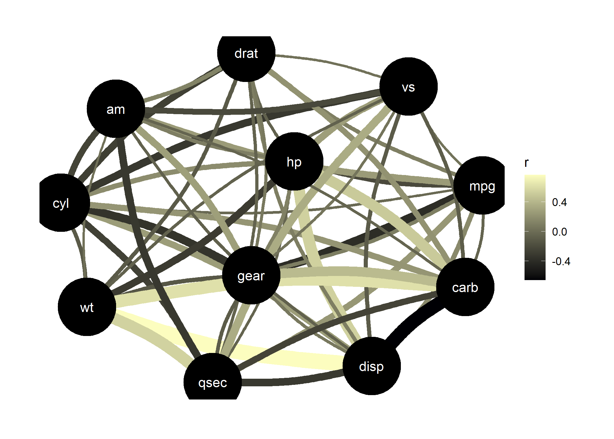
Such partial correlations can also be represented as Gaussian
Graphical Models (GGM), an increasingly popular tool in psychology. A
GGM traditionally include a set of variables depicted as circles
(“nodes”), and a set of lines that visualize relationships between them,
which thickness represents the strength of association (see Bhushan et
al.,
2019).

rCopy
library(see) # for plotting
library(ggraph) # needs to be loaded

plot(correlation(mtcars, partial = TRUE)) +
  scale_edge_color_continuous(low = "#000004FF", high = "#FCFDBFFF")

<!-- -->

Multilevel Correlations

It also provide some cutting-edge methods, such as Multilevel (partial)
correlations. These are are partial correlations based on linear
mixed-effects models that include the factors as random effects.
They can be see as correlations adjusted for some group
(hierarchical) variability.

rCopy
iris %>%
  correlation(partial = TRUE, multilevel = TRUE) %>%
  summary()
## # Correlation Matrix (pearson-method)
## 
## Parameter    | Petal.Width | Petal.Length | Sepal.Width
## -------------------------------------------------------
## Sepal.Length |      -0.17* |      0.71*** |     0.43***
## Sepal.Width  |     0.39*** |       -0.18* |            
## Petal.Length |     0.38*** |              |            
## 
## p-value adjustment method: Holm (1979)

However, if the partial argument is set to FALSE, it will try to
convert the partial coefficient into regular ones.These can be
converted back to full correlations:

rCopy
iris %>%
  correlation(partial = FALSE, multilevel = TRUE) %>%
  summary()
## Parameter    | Petal.Width | Petal.Length | Sepal.Width
## -------------------------------------------------------
## Sepal.Length |     0.36*** |      0.76*** |     0.53***
## Sepal.Width  |     0.47*** |      0.38*** |            
## Petal.Length |     0.48*** |              |

Contributing and Support

In case you want to file an issue or contribute in another way to the
package, please follow this
guide. For
questions about the functionality, you may either contact us via email
or also file an issue.

Code of Conduct

Please note that this project is released with a Contributor Code of
Conduct.
By participating in this project you agree to abide by its terms.