SCP
An end-to-end Single-Cell Pipeline designed to facilitate comprehensive analysis and exploration of single-cell data.
SCP provides a comprehensive set of tools for single-cell data processing and downstream analysis. The project is written primarily in R, distributed under the GNU General Public License v3.0 license, first published in 2022. Key topics include: anndata, scanpy, scatac-seq, scrna-pipeline, scrna-seq.
SCP: Single-Cell Pipeline
<!-- badges: start -->


SCP provides a comprehensive set of tools for single-cell data
processing and downstream analysis.
The package includes the following facilities:
- Integrated single-cell quality control methods.
- Pipelines embedded with multiple methods for normalization, feature
reduction, and cell population identification (standard Seurat
workflow). - Pipelines embedded with multiple integration methods for scRNA-seq or
scATAC-seq data, including Uncorrected,
Seurat,
scVI,
MNN,
fastMNN,
Harmony,
Scanorama,
BBKNN,
CSS,
LIGER,
Conos,
ComBat. - Multiple single-cell downstream analyses such as identification of
differential features, enrichment analysis, GSEA analysis,
identification of dynamic features,
PAGA, RNA
velocity,
Palantir,
Monocle2,
Monocle3, etc. - Multiple methods for automatic annotation of single-cell data and
methods for projection between single-cell datasets. - High-quality data visualization methods.
- Fast deployment of single-cell data into SCExplorer, a shiny
app that provides an interactive
visualization interface.
The functions in the SCP package are all developed around the Seurat
object and are compatible
with other Seurat functions.
R version requirement
- R >= 4.1.0
Installation in the global R environment
You can install the latest version of SCP from
GitHub with:
rif (!require("devtools", quietly = TRUE)) { install.packages("devtools") } devtools::install_github("zhanghao-njmu/SCP")
Create a python environment for SCP
To run functions such as RunPAGA or RunSCVELO, SCP requires
conda to create a
separate python environment. The default environment name is
"SCP_env". You can specify the environment name for SCP by setting
options(SCP_env_name="new_name")
Now, you can run PrepareEnv() to create the python environment for
SCP. If the conda binary is not found, it will automatically download
and install miniconda.
rSCP::PrepareEnv()
To force SCP to use a specific conda binary, it is recommended to set
reticulate.conda_binary R option:
roptions(reticulate.conda_binary = "/path/to/conda") SCP::PrepareEnv()
If the download of miniconda or pip packages is slow, you can specify
the miniconda repo and PyPI mirror according to your network region.
rSCP::PrepareEnv( miniconda_repo = "https://mirrors.bfsu.edu.cn/anaconda/miniconda", pip_options = "-i https://pypi.tuna.tsinghua.edu.cn/simple" )
Available miniconda repositories:
-
https://repo.anaconda.com/miniconda (default)
Available PyPI mirrors:
-
https://pypi.python.org/simple (default)
Installation in an isolated R environment using renv
If you do not want to change your current R environment or require
reproducibility, you can use the renv
package to install SCP into an isolated R environment.
Create an isolated R environment
rif (!require("renv", quietly = TRUE)) { install.packages("renv") } dir.create("~/SCP_env", recursive = TRUE) # It cannot be the home directory "~" ! renv::init(project = "~/SCP_env", bare = TRUE, restart = TRUE)
Option 1: Install SCP from GitHub and create SCP python environment
rrenv::activate(project = "~/SCP_env") renv::install("BiocManager") renv::install("zhanghao-njmu/SCP", repos = BiocManager::repositories()) SCP::PrepareEnv()
Option 2: If SCP is already installed in the global environment, copy
SCP from the local library
rrenv::activate(project = "~/SCP_env") renv::hydrate("SCP") SCP::PrepareEnv()
Activate SCP environment first before use
rrenv::activate(project = "~/SCP_env") library(SCP) data("pancreas_sub") pancreas_sub <- RunPAGA(srt = pancreas_sub, group_by = "SubCellType", linear_reduction = "PCA", nonlinear_reduction = "UMAP") CellDimPlot(pancreas_sub, group.by = "SubCellType", reduction = "draw_graph_fr")
Save and restore the state of SCP environment
rrenv::snapshot(project = "~/SCP_env") renv::restore(project = "~/SCP_env")
Quick Start
Data exploration
The analysis is based on a subsetted version of mouse pancreas
data.
rlibrary(SCP) library(BiocParallel) register(MulticoreParam(workers = 8, progressbar = TRUE)) data("pancreas_sub") print(pancreas_sub) #> An object of class Seurat #> 47874 features across 1000 samples within 3 assays #> Active assay: RNA (15958 features, 3467 variable features) #> 2 other assays present: spliced, unspliced #> 2 dimensional reductions calculated: PCA, UMAP
<img src="man/figures/EDA-1.png" width="100%" style="display: block; margin: auto;" />rCellDimPlot( srt = pancreas_sub, group.by = c("CellType", "SubCellType"), reduction = "UMAP", theme_use = "theme_blank" )
<img src="man/figures/EDA-2.png" width="100%" style="display: block; margin: auto;" />rCellDimPlot( srt = pancreas_sub, group.by = "SubCellType", stat.by = "Phase", reduction = "UMAP", theme_use = "theme_blank" )
<img src="man/figures/EDA-3.png" width="100%" style="display: block; margin: auto;" />rFeatureDimPlot( srt = pancreas_sub, features = c("Sox9", "Neurog3", "Fev", "Rbp4"), reduction = "UMAP", theme_use = "theme_blank" )
<img src="man/figures/EDA-4.png" width="100%" style="display: block; margin: auto;" />rFeatureDimPlot( srt = pancreas_sub, features = c("Ins1", "Gcg", "Sst", "Ghrl"), compare_features = TRUE, label = TRUE, label_insitu = TRUE, reduction = "UMAP", theme_use = "theme_blank" )
<img src="man/figures/EDA-5.png" width="100%" style="display: block; margin: auto;" />rht <- GroupHeatmap( srt = pancreas_sub, features = c( "Sox9", "Anxa2", # Ductal "Neurog3", "Hes6", # EPs "Fev", "Neurod1", # Pre-endocrine "Rbp4", "Pyy", # Endocrine "Ins1", "Gcg", "Sst", "Ghrl" # Beta, Alpha, Delta, Epsilon ), group.by = c("CellType", "SubCellType"), heatmap_palette = "YlOrRd", cell_annotation = c("Phase", "G2M_score", "Cdh2"), cell_annotation_palette = c("Dark2", "Paired", "Paired"), show_row_names = TRUE, row_names_side = "left", add_dot = TRUE, add_reticle = TRUE ) print(ht$plot)
CellQC
<img src="man/figures/RunCellQC-1.png" width="100%" style="display: block; margin: auto;" />rpancreas_sub <- RunCellQC(srt = pancreas_sub) CellDimPlot(srt = pancreas_sub, group.by = "CellQC", reduction = "UMAP")
<img src="man/figures/RunCellQC-2.png" width="100%" style="display: block; margin: auto;" />rCellStatPlot(srt = pancreas_sub, stat.by = "CellQC", group.by = "CellType", label = TRUE)
<img src="man/figures/RunCellQC-3.png" width="100%" style="display: block; margin: auto;" />rCellStatPlot( srt = pancreas_sub, stat.by = c( "db_qc", "outlier_qc", "umi_qc", "gene_qc", "mito_qc", "ribo_qc", "ribo_mito_ratio_qc", "species_qc" ), plot_type = "upset", stat_level = "Fail" )
Standard pipeline
<img src="man/figures/Standard_SCP-1.png" width="100%" style="display: block; margin: auto;" />rpancreas_sub <- Standard_SCP(srt = pancreas_sub) CellDimPlot( srt = pancreas_sub, group.by = c("CellType", "SubCellType"), reduction = "StandardUMAP2D", theme_use = "theme_blank" )
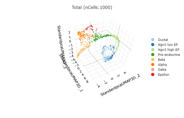
rCellDimPlot3D(srt = pancreas_sub, group.by = "SubCellType")
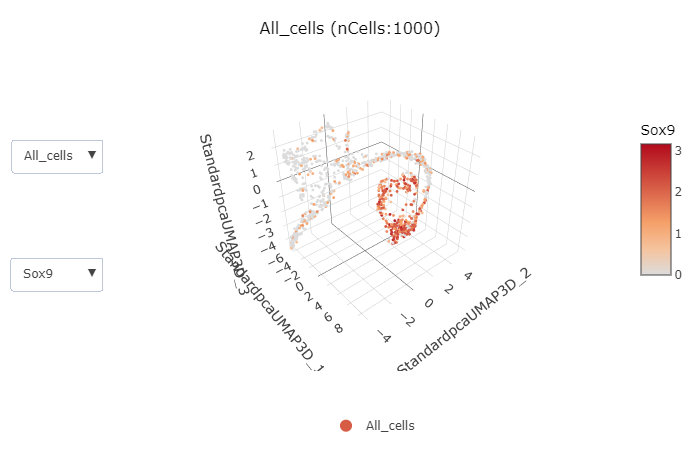
rFeatureDimPlot3D(srt = pancreas_sub, features = c("Sox9", "Neurog3", "Fev", "Rbp4"))
Integration pipeline
Example data for integration is a subsetted version of panc8(eight
human pancreas datasets)
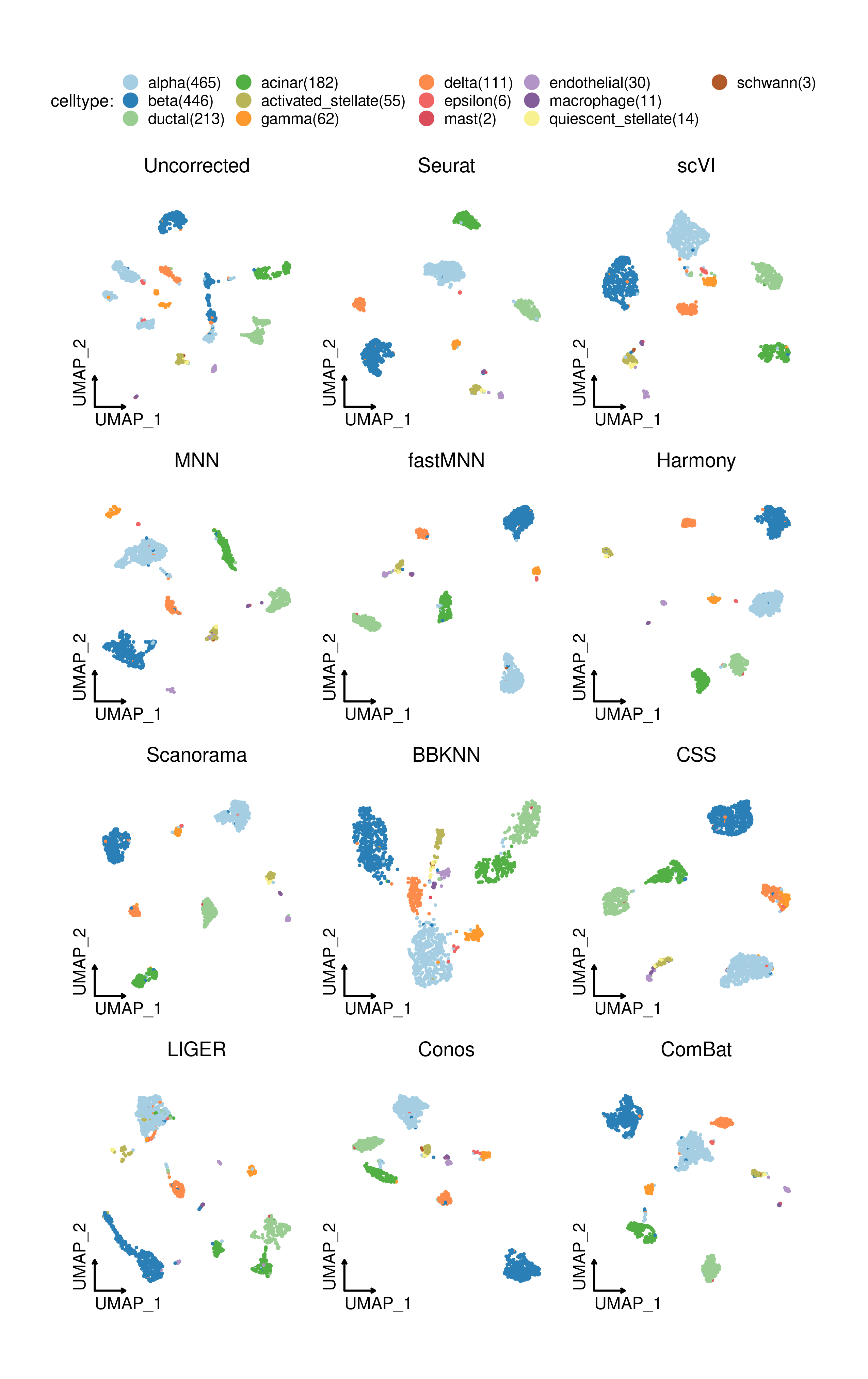
<img src="man/figures/Integration_SCP-1.png" width="100%" style="display: block; margin: auto;" />rdata("panc8_sub") panc8_sub <- Integration_SCP(srtMerge = panc8_sub, batch = "tech", integration_method = "Seurat") CellDimPlot( srt = panc8_sub, group.by = c("celltype", "tech"), reduction = "SeuratUMAP2D", title = "Seurat", theme_use = "theme_blank" )
UMAP embeddings based on different integration methods in SCP:
Cell projection between single-cell datasets
<img src="man/figures/RunKNNMap-1.png" width="100%" style="display: block; margin: auto;" />rpanc8_rename <- RenameFeatures( srt = panc8_sub, newnames = make.unique(capitalize(rownames(panc8_sub[["RNA"]]), force_tolower = TRUE)), assays = "RNA" ) srt_query <- RunKNNMap(srt_query = pancreas_sub, srt_ref = panc8_rename, ref_umap = "SeuratUMAP2D") ProjectionPlot( srt_query = srt_query, srt_ref = panc8_rename, query_group = "SubCellType", ref_group = "celltype" )
Cell annotation using bulk RNA-seq datasets
<img src="man/figures/RunKNNPredict-bulk-1.png" width="100%" style="display: block; margin: auto;" />rdata("ref_scMCA") pancreas_sub <- RunKNNPredict(srt_query = pancreas_sub, bulk_ref = ref_scMCA, filter_lowfreq = 20) CellDimPlot(srt = pancreas_sub, group.by = "KNNPredict_classification", reduction = "UMAP", label = TRUE)
Cell annotation using single-cell datasets
<img src="man/figures/RunKNNPredict-scrna-1.png" width="100%" style="display: block; margin: auto;" />rpancreas_sub <- RunKNNPredict( srt_query = pancreas_sub, srt_ref = panc8_rename, ref_group = "celltype", filter_lowfreq = 20 ) CellDimPlot(srt = pancreas_sub, group.by = "KNNPredict_classification", reduction = "UMAP", label = TRUE)
<img src="man/figures/RunKNNPredict-scrna-2.png" width="100%" style="display: block; margin: auto;" />rpancreas_sub <- RunKNNPredict( srt_query = pancreas_sub, srt_ref = panc8_rename, query_group = "SubCellType", ref_group = "celltype", return_full_distance_matrix = TRUE ) CellDimPlot(srt = pancreas_sub, group.by = "KNNPredict_classification", reduction = "UMAP", label = TRUE)
<img src="man/figures/RunKNNPredict-scrna-3.png" width="100%" style="display: block; margin: auto;" />rht <- CellCorHeatmap( srt_query = pancreas_sub, srt_ref = panc8_rename, query_group = "SubCellType", ref_group = "celltype", nlabel = 3, label_by = "row", show_row_names = TRUE, show_column_names = TRUE ) print(ht$plot)
PAGA analysis
<img src="man/figures/RunPAGA-1.png" width="100%" style="display: block; margin: auto;" />rpancreas_sub <- RunPAGA( srt = pancreas_sub, group_by = "SubCellType", linear_reduction = "PCA", nonlinear_reduction = "UMAP" ) PAGAPlot(srt = pancreas_sub, reduction = "UMAP", label = TRUE, label_insitu = TRUE, label_repel = TRUE)
Velocity analysis
To estimate RNA velocity, you need to have both “spliced” and
“unspliced” assays in your Seurat object. You can generate these
matrices using velocyto,
bustools,
or
alevin.
<img src="man/figures/RunSCVELO-1.png" width="100%" style="display: block; margin: auto;" />rpancreas_sub <- RunSCVELO( srt = pancreas_sub, group_by = "SubCellType", linear_reduction = "PCA", nonlinear_reduction = "UMAP" ) VelocityPlot(srt = pancreas_sub, reduction = "UMAP", group_by = "SubCellType")
<img src="man/figures/RunSCVELO-2.png" width="100%" style="display: block; margin: auto;" />rVelocityPlot(srt = pancreas_sub, reduction = "UMAP", plot_type = "stream")
Differential expression analysis
<img src="man/figures/RunDEtest-1.png" width="100%" style="display: block; margin: auto;" />rpancreas_sub <- RunDEtest(srt = pancreas_sub, group_by = "CellType", fc.threshold = 1, only.pos = FALSE) VolcanoPlot(srt = pancreas_sub, group_by = "CellType")
<img src="man/figures/FeatureHeatmap-1.png" width="100%" style="display: block; margin: auto;" />rDEGs <- pancreas_sub@tools$DEtest_CellType$AllMarkers_wilcox DEGs <- DEGs[with(DEGs, avg_log2FC > 1 & p_val_adj < 0.05), ] # Annotate features with transcription factors and surface proteins pancreas_sub <- AnnotateFeatures(pancreas_sub, species = "Mus_musculus", db = c("TF", "CSPA")) ht <- FeatureHeatmap( srt = pancreas_sub, group.by = "CellType", features = DEGs$gene, feature_split = DEGs$group1, species = "Mus_musculus", db = c("GO_BP", "KEGG", "WikiPathway"), anno_terms = TRUE, feature_annotation = c("TF", "CSPA"), feature_annotation_palcolor = list(c("gold", "steelblue"), c("forestgreen")), height = 5, width = 4 ) print(ht$plot)
Enrichment analysis(over-representation)
<img src="man/figures/RunEnrichment-1.png" width="100%" style="display: block; margin: auto;" />rpancreas_sub <- RunEnrichment( srt = pancreas_sub, group_by = "CellType", db = "GO_BP", species = "Mus_musculus", DE_threshold = "avg_log2FC > log2(1.5) & p_val_adj < 0.05" ) EnrichmentPlot( srt = pancreas_sub, group_by = "CellType", group_use = c("Ductal", "Endocrine"), plot_type = "bar" )
<img src="man/figures/RunEnrichment-2.png" width="100%" style="display: block; margin: auto;" />rEnrichmentPlot( srt = pancreas_sub, group_by = "CellType", group_use = c("Ductal", "Endocrine"), plot_type = "wordcloud" )
<img src="man/figures/RunEnrichment-3.png" width="100%" style="display: block; margin: auto;" />rEnrichmentPlot( srt = pancreas_sub, group_by = "CellType", group_use = c("Ductal", "Endocrine"), plot_type = "wordcloud", word_type = "feature" )
<img src="man/figures/RunEnrichment-4.png" width="100%" style="display: block; margin: auto;" />rEnrichmentPlot( srt = pancreas_sub, group_by = "CellType", group_use = "Ductal", plot_type = "network" )
To ensure that labels are visible, you can adjust the size of the
viewer panel on Rstudio IDE.
<img src="man/figures/Enrichment_enrichmap-1.png" width="100%" style="display: block; margin: auto;" />rEnrichmentPlot( srt = pancreas_sub, group_by = "CellType", group_use = "Ductal", plot_type = "enrichmap" )
<img src="man/figures/Enrichment_comparison-1.png" width="100%" style="display: block; margin: auto;" />rEnrichmentPlot(srt = pancreas_sub, group_by = "CellType", plot_type = "comparison")
Enrichment analysis(GSEA)
<img src="man/figures/RunGSEA-1.png" width="100%" style="display: block; margin: auto;" />rpancreas_sub <- RunGSEA( srt = pancreas_sub, group_by = "CellType", db = "GO_BP", species = "Mus_musculus", DE_threshold = "p_val_adj < 0.05" ) GSEAPlot(srt = pancreas_sub, group_by = "CellType", group_use = "Endocrine", id_use = "GO:0007186")
<img src="man/figures/GSEA_bar-1.png" width="100%" style="display: block; margin: auto;" />rGSEAPlot( srt = pancreas_sub, group_by = "CellType", group_use = "Endocrine", plot_type = "bar", direction = "both", topTerm = 20 )
<img src="man/figures/GSEA_comparison-1.png" width="100%" style="display: block; margin: auto;" />rGSEAPlot(srt = pancreas_sub, group_by = "CellType", plot_type = "comparison")
Trajectory inference
<img src="man/figures/RunSlingshot-1.png" width="100%" style="display: block; margin: auto;" />rpancreas_sub <- RunSlingshot(srt = pancreas_sub, group.by = "SubCellType", reduction = "UMAP")
<img src="man/figures/RunSlingshot-2.png" width="100%" style="display: block; margin: auto;" />rFeatureDimPlot(pancreas_sub, features = paste0("Lineage", 1:3), reduction = "UMAP", theme_use = "theme_blank")
<img src="man/figures/RunSlingshot-3.png" width="100%" style="display: block; margin: auto;" />rCellDimPlot(pancreas_sub, group.by = "SubCellType", reduction = "UMAP", lineages = paste0("Lineage", 1:3), lineages_span = 0.1)
Dynamic features
<img src="man/figures/DynamicHeatmap-1.png" width="100%" style="display: block; margin: auto;" />rpancreas_sub <- RunDynamicFeatures(srt = pancreas_sub, lineages = c("Lineage1", "Lineage2"), n_candidates = 200) ht <- DynamicHeatmap( srt = pancreas_sub, lineages = c("Lineage1", "Lineage2"), use_fitted = TRUE, n_split = 6, reverse_ht = "Lineage1", species = "Mus_musculus", db = "GO_BP", anno_terms = TRUE, anno_keys = TRUE, anno_features = TRUE, heatmap_palette = "viridis", cell_annotation = "SubCellType", separate_annotation = list("SubCellType", c("Nnat", "Irx1")), separate_annotation_palette = c("Paired", "Set1"), feature_annotation = c("TF", "CSPA"), feature_annotation_palcolor = list(c("gold", "steelblue"), c("forestgreen")), pseudotime_label = 25, pseudotime_label_color = "red", height = 5, width = 2 ) print(ht$plot)
<img src="man/figures/DynamicPlot-1.png" width="100%" style="display: block; margin: auto;" />rDynamicPlot( srt = pancreas_sub, lineages = c("Lineage1", "Lineage2"), group.by = "SubCellType", features = c("Plk1", "Hes1", "Neurod2", "Ghrl", "Gcg", "Ins2"), compare_lineages = TRUE, compare_features = FALSE )
<img src="man/figures/FeatureStatPlot-1.png" width="100%" style="display: block; margin: auto;" />rFeatureStatPlot( srt = pancreas_sub, group.by = "SubCellType", bg.by = "CellType", stat.by = c("Sox9", "Neurod2", "Isl1", "Rbp4"), add_box = TRUE, comparisons = list( c("Ductal", "Ngn3 low EP"), c("Ngn3 high EP", "Pre-endocrine"), c("Alpha", "Beta") ) )
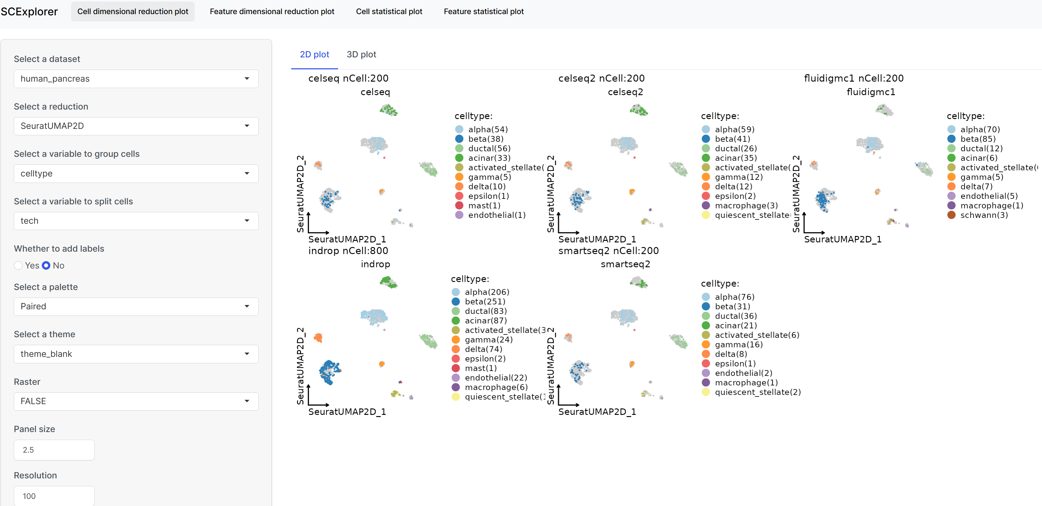
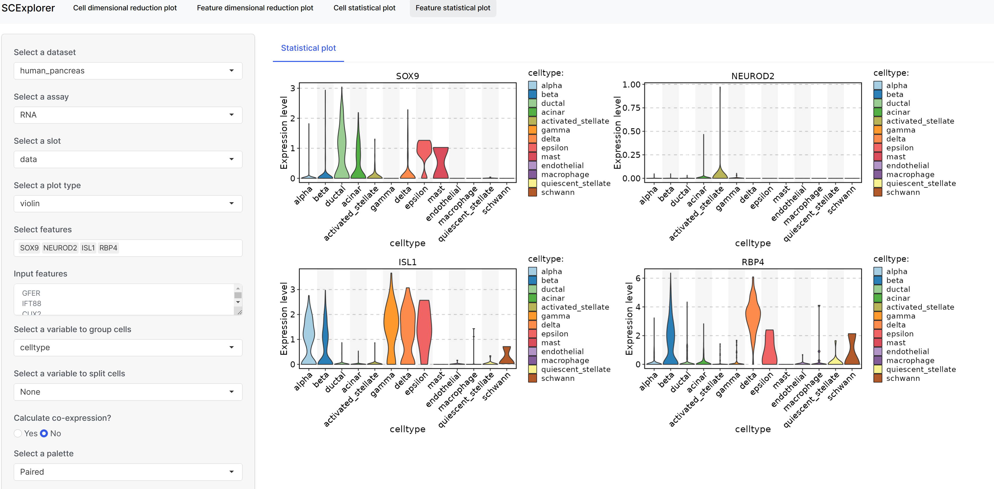
Interactive data visualization with SCExplorer
rPrepareSCExplorer(list(mouse_pancreas = pancreas_sub, human_pancreas = panc8_sub), base_dir = "./SCExplorer") app <- RunSCExplorer(base_dir = "./SCExplorer") list.files("./SCExplorer") # This directory can be used as site directory for Shiny Server. if (interactive()) { shiny::runApp(app) }
Other visualization examples
CellDimPlot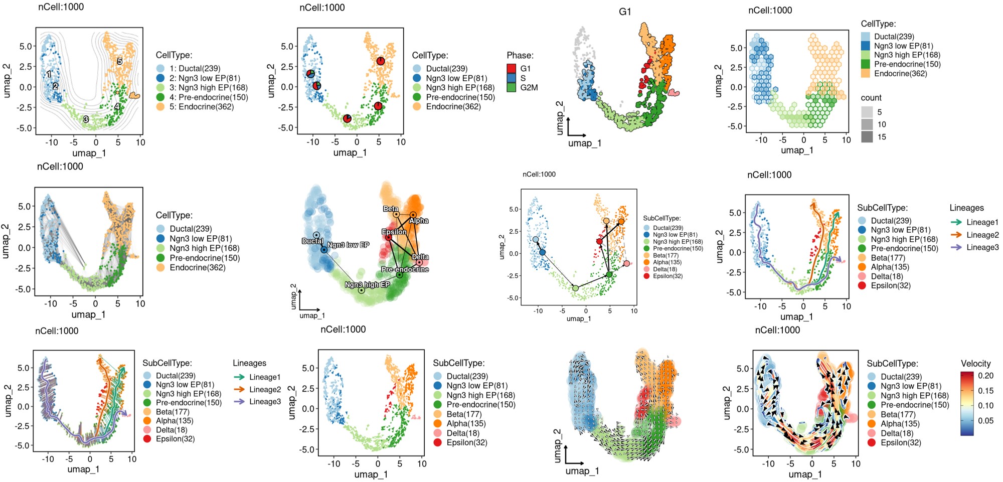
CellStatPlot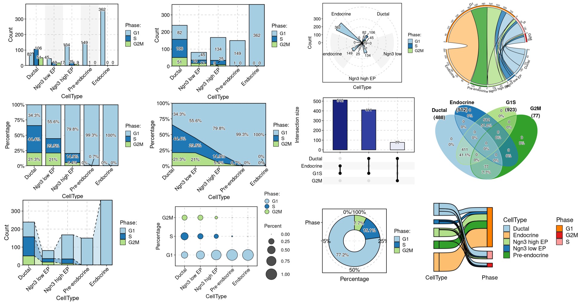
FeatureStatPlot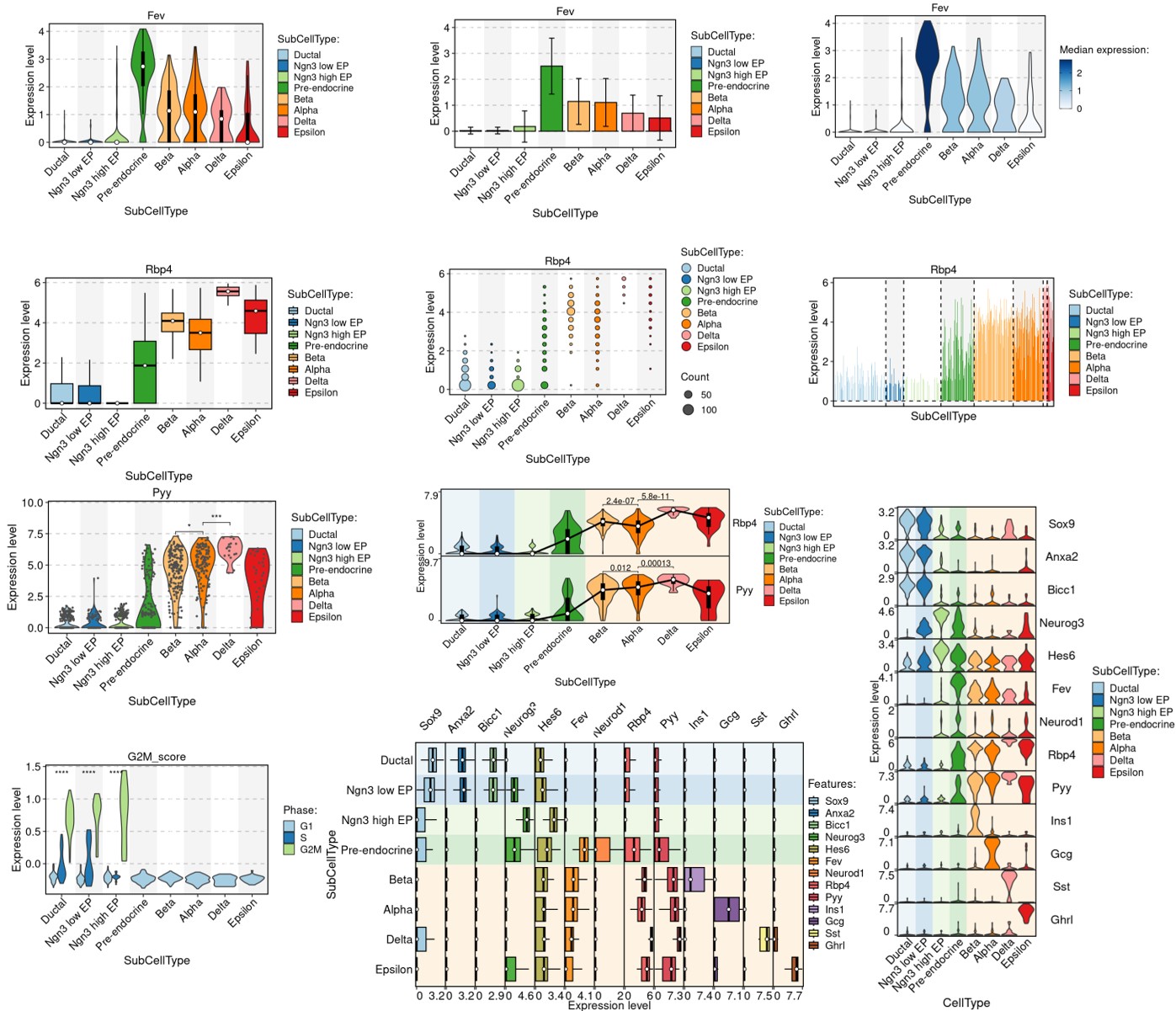
GroupHeatmap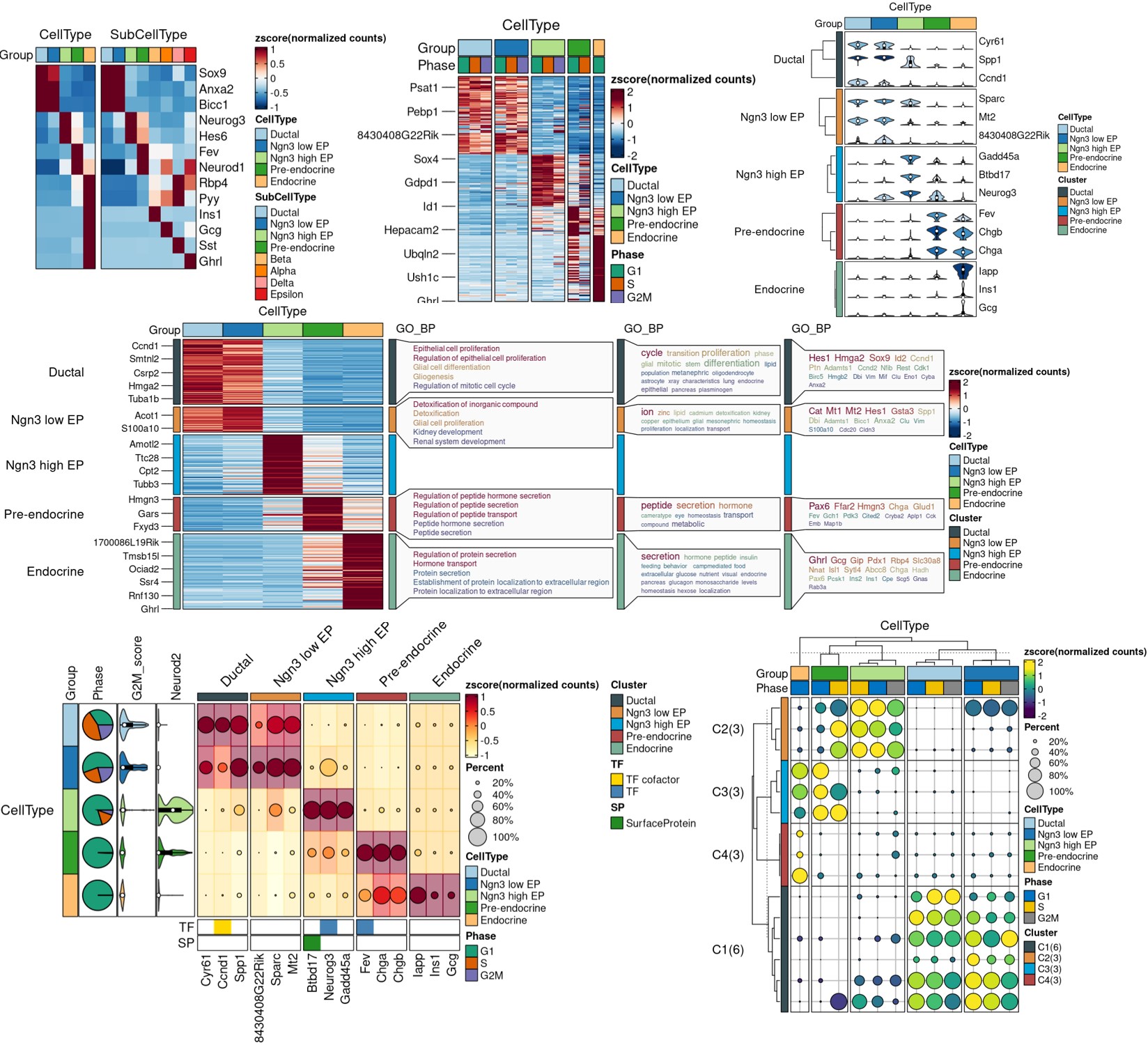
You can also find more examples in the documentation of the function:
Integration_SCP,
RunKNNMap,
RunMonocle3,
RunPalantir,
etc.
Contributors
Showing top 1 contributor by commit count.

Related Repositories

scverse/scanpy
Single-cell analysis in Python. Scales to >100M cells.
scverse/anndata
Annotated data.
scverse/rapids-singlecell
rapids-singlecell: GPU-accelerated framework for scRNA analysis
scverse/muon
muon is a multimodal omics Python framework
scverse/anndataR
AnnData interoperability in R

basilkhuder/Seurat-to-RNA-Velocity
A guide to using a Seurat object in conjunction with RNA Velocity